resample

1. The Importance of Resampling

In machine learning, we want to build models that generalize well to new, unseen data. A common mistake is to train and evaluate a model on the same dataset. This often leads to overfitting, where the model learns the noise in the training data, not the underlying pattern. As a result, the model performs well on the data it has seen but fails miserably on new data.

Resampling is a collection of techniques used to combat this. It involves repeatedly drawing samples from a training set and refitting a model on each sample. This process allows us to:

• Estimate model performance: Get a more accurate and robust estimate of how the model will perform on unseen data.
• Understand variability: See how much the model’s performance changes across different subsets of the data.
• Tune hyperparameters: Find the best settings for a model by evaluating them across multiple validation sets.

The rsample package, part of the tidymodels ecosystem, provides a consistent and intuitive interface for creating different types of resamples.

library(rsample)
library(tidyverse)

# We will use the iris dataset for demonstration
data(iris)

2. k-Fold Cross-Validation (CV)

This is the most common resampling method. The data is randomly split into k equal-sized partitions (or “folds”). For each fold, the model is trained on the other k-1 folds (the analysis set) and tested on the held-out fold (the assessment set). The process is repeated k times, with each fold serving as the test set exactly once. The final performance is the average of the performances across all k folds.

vfold_cv() creates the folds. A v of 10 is a common choice.

k_fold_resample <- vfold_cv(iris, v = 10)
k_fold_resample

#  10-fold cross-validation 
# A tibble: 10 × 2
   splits           id    
   <list>           <chr> 
 1 <split [135/15]> Fold01
 2 <split [135/15]> Fold02
 3 <split [135/15]> Fold03
 4 <split [135/15]> Fold04
 5 <split [135/15]> Fold05
 6 <split [135/15]> Fold06
 7 <split [135/15]> Fold07
 8 <split [135/15]> Fold08
 9 <split [135/15]> Fold09
10 <split [135/15]> Fold10

Each row in the output represents one fold. The <split> column contains rsplit objects, which are lightweight pointers to the actual data for the training (analysis) and testing (assessment) sets for that fold.

Working with rsplit objects

You can extract the analysis and assessment data for a specific split.

# Get the first split object
first_split <- k_fold_resample$splits[[1]]

# Get the training data for the first fold
analysis_data <- analysis(first_split)

# Get the testing data for the first fold
assessment_data <- assessment(first_split)

cat(paste("Analysis (training) rows:", nrow(analysis_data), "\n"))

Analysis (training) rows: 135 

cat(paste("Assessment (testing) rows:", nrow(assessment_data), "\n"))

Assessment (testing) rows: 15 

3. Monte Carlo Cross-Validation (MCCV)

MCCV, also known as repeated random sub-sampling validation, involves randomly splitting the data into a training and a validation set a specified number of times. Unlike k-fold CV, the assessment sets are not mutually exclusive and can overlap.

This method is useful when you want to control the size of the validation set directly, rather than being constrained by the number of folds. It can be more computationally intensive than k-fold CV if many repetitions are used.

mc_cv() creates the splits. prop is the proportion of data to be used for training, and times is the number of splits to create.

mc_resample <- mc_cv(iris, prop = 9/10, times = 20)
mc_resample

# Monte Carlo cross-validation (0.9/0.1) with 20 resamples 
# A tibble: 20 × 2
   splits           id        
   <list>           <chr>     
 1 <split [135/15]> Resample01
 2 <split [135/15]> Resample02
 3 <split [135/15]> Resample03
 4 <split [135/15]> Resample04
 5 <split [135/15]> Resample05
 6 <split [135/15]> Resample06
 7 <split [135/15]> Resample07
 8 <split [135/15]> Resample08
 9 <split [135/15]> Resample09
10 <split [135/15]> Resample10
11 <split [135/15]> Resample11
12 <split [135/15]> Resample12
13 <split [135/15]> Resample13
14 <split [135/15]> Resample14
15 <split [135/15]> Resample15
16 <split [135/15]> Resample16
17 <split [135/15]> Resample17
18 <split [135/15]> Resample18
19 <split [135/15]> Resample19
20 <split [135/15]> Resample20

4. The Bootstrap

A bootstrap sample is created by sampling from the original dataset with replacement. The resulting sample is the same size as the original dataset. Because of sampling with replacement, some data points will be selected multiple times, while others will not be selected at all (these are called the “out-of-bag” samples).

Bootstrapping is useful for estimating the uncertainty of a statistic (like a model coefficient) and is the foundation for ensemble methods like Random Forest. The out-of-bag sample can be used as a validation set.

bootstraps() creates the bootstrap samples.

bootstraps_resample <- bootstraps(iris, times = 1000)
bootstraps_resample

# Bootstrap sampling 
# A tibble: 1,000 × 2
   splits           id           
   <list>           <chr>        
 1 <split [150/58]> Bootstrap0001
 2 <split [150/52]> Bootstrap0002
 3 <split [150/58]> Bootstrap0003
 4 <split [150/56]> Bootstrap0004
 5 <split [150/57]> Bootstrap0005
 6 <split [150/55]> Bootstrap0006
 7 <split [150/53]> Bootstrap0007
 8 <split [150/56]> Bootstrap0008
 9 <split [150/55]> Bootstrap0009
10 <split [150/58]> Bootstrap0010
# ℹ 990 more rows

5. Stratified Sampling

When dealing with a classification problem where the outcome variable is imbalanced (i.e., some classes have very few samples), random splitting can lead to folds where one or more classes are missing entirely from the training or testing set.

Stratified sampling ensures that the class distribution in each fold is approximately the same as in the original dataset. You can do this by specifying the strata argument in the resampling functions. This is highly recommended for classification problems.

# Create 10-fold cross-validation splits, stratified by the Species column
stratified_k_fold <- vfold_cv(iris, v = 10, strata = Species)
stratified_k_fold

#  10-fold cross-validation using stratification 
# A tibble: 10 × 2
   splits           id    
   <list>           <chr> 
 1 <split [135/15]> Fold01
 2 <split [135/15]> Fold02
 3 <split [135/15]> Fold03
 4 <split [135/15]> Fold04
 5 <split [135/15]> Fold05
 6 <split [135/15]> Fold06
 7 <split [135/15]> Fold07
 8 <split [135/15]> Fold08
 9 <split [135/15]> Fold09
10 <split [135/15]> Fold10

6. Visualizing Resamples

It can be helpful to visualize the resamples to understand how the data is being split. The code below defines a helper function to plot the distribution of a variable across the different resample splits.

# Helper function to extract and plot data from splits
plot_resample_dist <- function(resample_obj, variable) {
  resample_obj %>% 
    mutate(fold_id = as.character(row_number())) %>% 
    pull(splits) %>% 
    map_dfr(~as_tibble(analysis(.)), .id = "fold_id") %>% 
    ggplot(aes(x = {{variable}}, fill = fold_id)) + 
    geom_density(alpha = 0.5, show.legend = FALSE) + 
    labs(
      title = paste("Distribution of", rlang::as_name(enquo(variable)), "across resamples"),
      x = rlang::as_name(enquo(variable)),
      y = "Density"
    ) + 
    theme_minimal()
}

# Visualize the distribution of Sepal.Length across the k-fold splits
plot_resample_dist(k_fold_resample, Sepal.Length)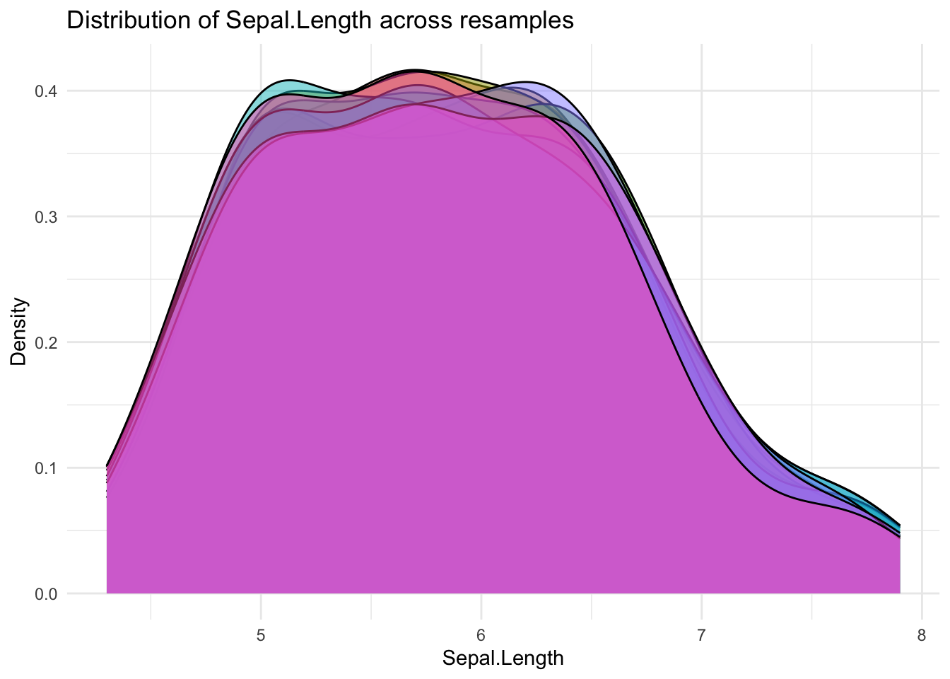

This visualization helps confirm that the splits are reasonably balanced and representative of the overall data distribution.